Statistics, Probability and Noise in DSP published: 20th February 2025
After working on my simple 8 step sequencer which only generates a gate signal for each active step in the sequence I wanted to add the functionality to generate control voltage for modulating the pitch for each active step. It's not much of a sequencer if it cannot generate pitch control voltage to make melodies. This is where things got tricky since I have a Daisy Pod which has an AC coupled audio output. What does that even mean? Well everything in modular synthesis is simply variations in voltage. Some are AC like the audio and some are DC like control voltage. The reason why modular is so flexible and intuitive because it's only voltages flowing through the system and the same voltage can be used for audio generation or modulating some aspect of the audio. Daisy Pod has an AC coupled audio so it cannot generate DC voltages since AC coupled outputs have a capacitor in series with the output and any DC component of the voltage is blocked while only allowing AC components. To generate a pitch control voltage I should be able to generate a voltage of let's say 1V and be able to sustain it till the next active step in the sequence. Ok but why only DC? Why can't we use AC to generate the control voltage, it's voltage after all? Let's say you want to control the pitch of an oscillator and if you were to use AC coupling the control voltage would constantly return to 0V since AC alternates between positive and negative from a reference point which is 0V. So using AC for control voltage would lead to your pitch decaying and coming back to its original pitch. AC coupled devices have a capacitor in series with the output. A capacitor is so called because it has a capacity to store energy and is made of two conductive plates separated by an insulator or a dielectric. Dielectrics are materials possessing high electrical resistivities and a good dielectric is therefore a good insulator. A capacitor is a little like a battery. Although they work in different ways capacitors and batteries store electrical energy. However, a battery generates and stores energy while a capacitor only stores the energy. Once you apply a voltage to the capacitor it starts to charge up and as soon as it charges fully no more current can flow through it and if the voltage is DC capacitor will block the passage of the voltage since it's now fully charged. A capacitor responds to AC by continuously charging and discharging when the input voltage swings positive, electrons flow one way building up charge, but before the capacitor can fully charge, the AC voltage swings negative, causing electrons to flow in the opposite direction. This constant reversal of voltage creates continuous electron movement in the circuit. The capacitor does not BLOCK anything, it just recreates the voltage at its input and the next part in the circuit uses that to create current flow based on the voltage changes.
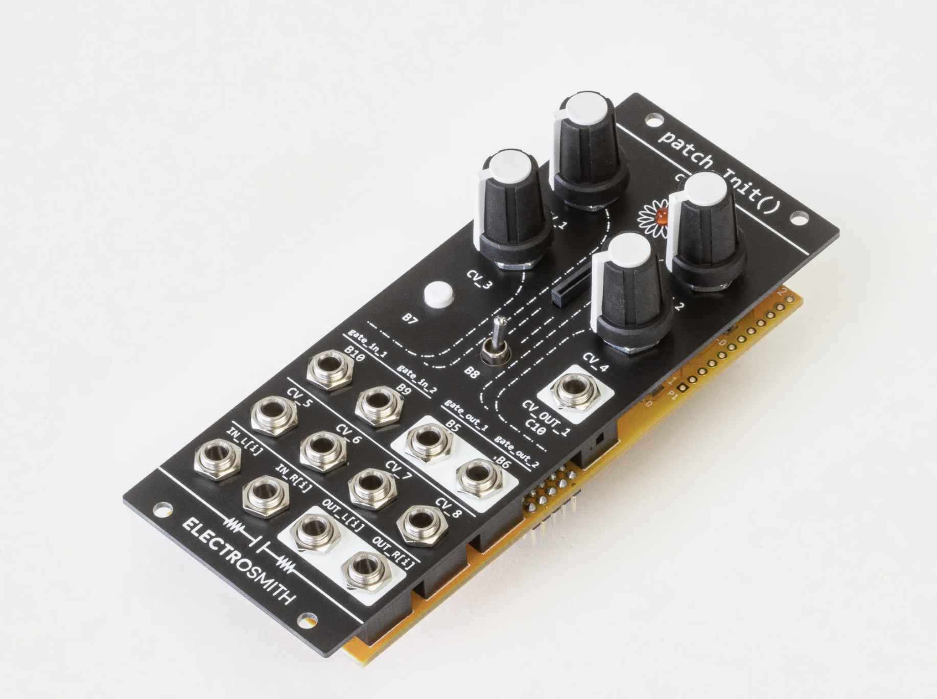
Ok so Daisy Pod has a DC coupled output so I cannot generate a pitch control voltage, what do I do now? Electro Smith the company who makes the Daisy Pod also makes other DSP modules. One of them is a Patch.init() module. This module's output is DC coupled which means it can pass both AC and DC voltages.
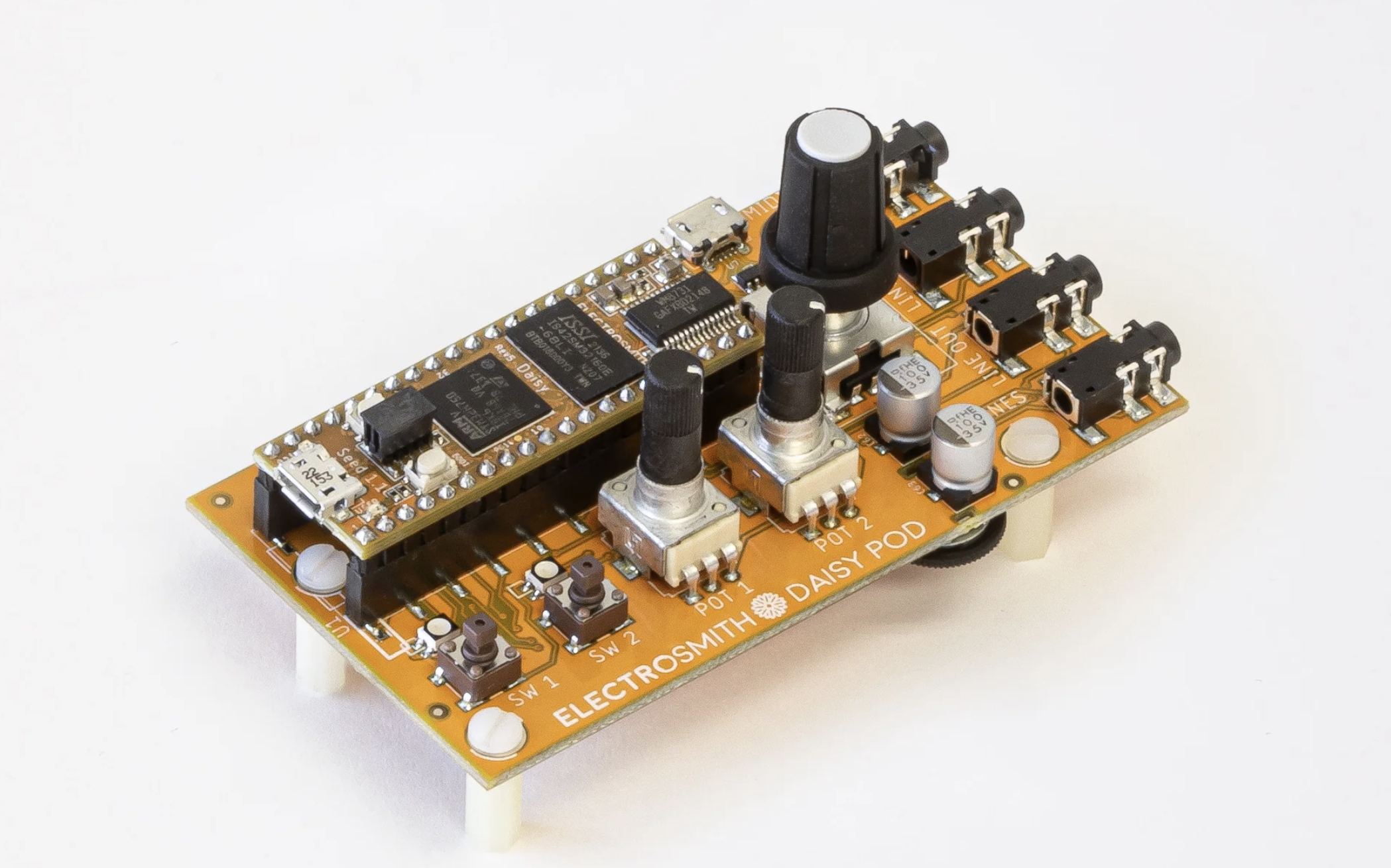
But this does not have some controls like an encoder, multiple LEDs, toggle switches which is in Daisy Pod so to make my step sequencer I had to split the functionality between these two modules. Here is the setup:
- In Daisy Pod use the encoder to step through the sequence. Use the toggle switch to turn on/off a step in the sequence. Use the knob1 to control the tempo and knob2 to set a pitch for the active step in the sequence. Pod will generate the gate signal for each active step in the sequence. It will also generate an audio signal for the pitch selected for the step.
- Patch.init() will take the gate signal and the audio signal. It will forward the gate signal to my Moog Mavis gate input which will trigger its VCA. It will calculate the frequency of the incoming audio signal and turn that frequency to a voltage based on the 1V/Octave standard. This control voltage will then be fed to Moog Mavis 1V/OCT input to control the pitch of the oscillator.
Since Patch.init() audio output is DC coupled I can easily generate
a pitch control voltage bt since it does not have enough hardware
controls I am using the Pod to do half of the work. The tricky part
here is calculating the frequency of the incoming audio signal and
converting it to a pitch control voltage. I have spent a couple of
days in getting the calculations right but so far I am not able to
get the frequency calculation right and I observed that I kept
making a lot of mistakes in my code and was often in completely
wrong direction.
Rather than continuing to struggle with code, I realized I needed to
step back and rebuild my foundation in Digital Signal Processing
concepts. Without solid DSP fundamentals, I was trying to solve
problems I didn't fully understand.
That was a brief of writing this article and let's get started
understanding some basic concepts needed to work with DSP.
Digital Signal Processing is a vast field with many different
applications. I am using DSP primarily for working with audio
signals. Ok so what is a signal? A signal is just a description of
how one parameter is related to another. An audio signal is just
voltage that varies over time. It's a continuous voltage signal that
represents how air pressure will change with respect to change in
electric potential of the voltage over time. Since both the
parameters can assume continuous range of values, it is called a
continuous signal. In comparison passing the signal through a
digital system forces each of the parameters to be
quantised. Quantising is the process
mapping a continuous range of analog values to a finite set of
digital values. This is called a discrete or digitised signal. For
an audio signal the quantisation can be done with an Analog to
Digital Converter (ADC). The ADC has a fixed number of resolution or
bits. If we have a 12 bit ADC we now have a 212 possible
set of values to represent each value in the signal. If you have a
5V signal with a 12 bit ADC you can detect the smallest voltage of
approximately 1.22mV.
5V/212 = 0.001220703125
Any voltage differences less than 1.22mV will be lost in the
quantisation. [this can be explained separately in different article
since it's quite an important concept]
If we were to plot a graph of the discrete signal the vertical axis
can represent any parameter like sound pressure, voltage, etc. This
parameter is called with other names:
the dependent variable, the range and the ordinate. The horizontal axis represents the other parameter of the signal
going by names:
the independent variable, the domain, the abscissa. The two parameters that form the signal are not interchangeable.
The parameter on the Y axis is said to be a function of the X axis.
The independent variables tells when and how the samples were taken
while the dependent variable is the actual measurement. Given a
value on the X axis we can always find the respective Y axis value
but usually not the other way around.
In DSP if a signal uses time as the independent variable then it is
said to be in the time domain. Just like that if the independent
variable is the frequency it is said to be in the frequency domain.
The type of the parameter on the X axis makes it the domain of the
signal.
Signal vs the underlying process
Let's play a probability game. We will create a signal out of
flipping a coin and noting down its outcome. Let's we will flip our
coin a 1000 times and generate a signal based on heads or tails. If
the outcome is head the sample value is one and if tails the sample
value is 0. The outcome here is 50/50 heads and tails. Each
individual flip has an expected value of 0.5 which comes from this
formula:
(probability of heads x value of heads) + (probability of tails x
value of tails). If you were to calculate the mean of the coin flip you'll get the
mean as 0.5. This is the mean of the
underlying process that helps generate
our signal. But if you were to actually generate a signal and
calculate its mean it is unlikely that it will have a mean of
exactly 0.5. If you were to do a 1000 coin flips you'll find out
that the outcome is not 500 heads and 500 tails. Due to the inherent
nature of how particles behave and tiny changes in the air pressure,
thermal vibrations of the atoms in the coin, the air bouncing off
the coin, etc. will introduce randomness in the outcome. This
introduces the quantum uncertainty in each coin flip. Getting an
equal outcome of heads and tails on coin flips is really rare.
The probabilities of the underlying process (the coin flip) are
constant but the statistics of the acquired signal changes each
time the experiment is repeated.
This randomness and the irregularity that we find in the actual data
is called: statistical variation, statistical fluctuation or
statistical noise. So now you have a signal which has error in it so
when you process it you'll come across issues like voltage level
might be higher ot lower than the true value, jitters in the signal,
and a bunch of other problems in your calculations. So how do we fix
it?
Statistics is the science of interpreting numerical data such as an
acquired signal. While probability is used to understand the
processes that generates that signal. To fix the statistical noise
we can use techniques like calculating the mean and standard
deviation of the acquired sample forming the signal. In electronics
the mean is called the DC value while AC refers to how the signal
fluctuates around the mean value. If the signal is a simple one like
a square or a sine wave its fluctuation can be described by its peak
to peak amplitude. But most real life signals are not symmetric like
that and have a well defined peak to peak value. So a generalised
approach needs to be applied for such signals. Standard deviation is
a measure of how much a sample deviates from its mean denoted by the
Greek Sigma notation σ.
To calculate how far the ith sample deviates from the
mean we can use the formula |xi
- μ|. Then the average deviation can be calculated by summing all
the individual deviations. We also use the absolute value of the
deviation otherwise positive and negative deviations would sum out
to zero. But the average deviation is not in statistics since it
does not fit with how signal physics works. Imagine the sound coming
out of a speaker. The sound is generated by the speaker's diaphragm
pushing outward and then inward from a center point. If we were to
average out the diaphragm movement we'd reach a number closer to
zero. If the average displacement of the diaphragm is zero how can
it produce any sound? We are able to hear the sound coming from the
speaker but statistically it's average is zero so there is
definitely something wrong with our statistics here. So average
deviation cannot be used here to make a correct estimation. That's
where standard deviation comes in. What matters in statistics is not
the deviation from the mean but the
power of the deviation of the mean and
standard deviation helps us calculate that correctly.
SD uses the signal power instead of the signal amplitude to
calculate the deviation by first squaring the value (power ∝
voltage2). Squaring is needed to make the values absolute
which gives us the power of the deviation of that value from the
mean. Squaring matches how things work in nature. For eg. if you
push something twice as hard you don't get twice the energy, you
actually get four times the energy. Then summing all the values and
calculating an average then and taking a square root to compensate
for the first squaring. The formula for standard deviation is:
hhhmmm something does not look right! Why are we dividing by N-1 when we have N samples? When we take a sample out of a population for statistical measures the data always contains error. Remember the statistical noise mentioned above in the article. The error is represented as:
Since N is in the denominator and if N is a small number the statistical noise will be large enough to throw our calculations away from the actual mean which means we do not have enough samples to characterise the process. Larger the value of N smaller the statistical noise. The law of large numbers guarantees the error becomes zero as N approaches infinity. Enter Bessel's Correction. Friedrich Wilhelm Bessel was a German mathematician among other things and he suggested using N - 1 instead of N which corrects the bias in a sample of population. When you have a finite set of sample from a given population, calculating a parameter like SD will not yield to a correct value. When you're working with a sample you've only got a small fraction of the population to work with. Your calculations are not going to be as accurate as they would have been if you had full entire set of data to work with.
μ -> population mean
Any x value in your sample is closer to x̄ than it is to μ. The sample mean is always smaller than the actual population mean. Dividing by N-1 instead of N moves the mean closer to the population mean. If N is large enough the N-1 difference does not matter, if N is small the replacement to N-1 provides an accurate estimate of the standard deviation of the underlying process. Division by N gives us the SD of the acquired signal and division by N-1 gives us the SD of the underlying process.
The Histogram, Probability Mass function, and Probability Distribution function
Let's take an Analog to Digital converter of 8 bits and acquire an audio signal. For this signal we collect 256000 samples. Since the ADC is 8 bits (28 = 256) each value of sample will be one of 246 possibilities from 0-255. Let's plot one part of the data set in the signal. The amplitude here represents what is the value the sample from 0-255 since we acquired signal from an 8 bit ADC. It's called "amplitude" because that's the standard term used in signal processing to describe the magnitude or value of a signal at any given point.
A histogram displays the number of samples there are in the signal that have values ranging from 0-127. So Y axis represents the number of occurrences of the value and X axis represents the value of the sample.
The histogram shows that there are 7 samples that have a value of
135, 7 samples that have a value of 131, etc. Let's call the
histogram Hi where
i is an index running from 0 to M-1
where M is the number of possible values each sample can take on.
Let's go and plot the complete sample and see what that looks like:
As you can see the larger the number of samples the smoother the curve is. Just like mean the statistical noise of the histogram is inversely proportional to the square root of the of number of samples used. So if you were to sum all the values of the histogram it must be equal to the number of samples in the signal. The formulas for mean and standard deviation are:
Statistics for the plotted data calculated using Histogram:
- Mean:
- Standard Deviation:
Using the histogram to calculate the SD is more efficient since in a
Histogram sampled with the same values are grouped together which
allows the statistics to be calculated by working with few numbers
rather than going through each sample in a very large data set. The
Histogram algorithm only does indexing and incrementing while the mean
and SD need to do addition and multiplication hence the Histogram
algorithm much faster.
But remember the acquired signal has statistical noise since an
acquired signal is a noisy version of the underlying process so we
need different names to represent our statistics. A Histogram is for
the acquired signal and the corresponding curve for the underlying
process is called the Probability Mass Function. A
Histogram is calculated with a finite set of data while PMF can be
estimated from the Histogram. The PMF tells us the probability of a
certain value being generated. Each value in the histogram is divided
by the total number of samples to approximate the PMF. So the Y axis
is a fractional value and if you were to add it up it will equal to
one.
PMF and Histogram can only be used with discrete data like a digitised signal in a computer. Probability Distribution Function is used to represent continuous signals like the ones in analog circuits. Imagine the audio signal passing through a modular synthesiser, for simplicity we will assume that a max voltage of 255 millivolts is passing through the system. It's plot would look something like this:
Remember PDF works with continuous signals so let's say a PDF of 0.029
at 129.25 does not mean there is a 3% chance that the signal will be
at 129.25 millivolts. The probability of the signal being 129.25
millivolts is infinitesimally small since there are infinite number of
values where the signal can be eg. 129.248888, 129.248889, 129.248890,
etc. For it to be exactly 129.25000 is really rare.
For continuous signal the values are stored in fractions so there
could be billions of possibilities to represent the value of a signal
at a point. Not just that most of the possible levels would have no
sample too. For eg. a 10000 sample signal with each sample having one
billion possible values would result in a histogram of one billion
data points but 10000 of them having a sample of zero. Each sample
must go into exactly one bin. When you're creating a histogram: you
have 10000 samples total, each sample must be placed in exactly one
bin, and each sample contributes a count of 1 to its bin. Therefore,
the total sum of all bin counts must equal your total number of
samples (10000). Such problems with large data sets can be fixed with
a technique called binning. In binning we
arbitrarily select the length of the histogram to a convenient number
like 1000 and call it a bin. For eg. imagine a signal with floating
point numbers from 0 to 10 with a histogram of say 1000 bins. This
means that bin 1 contains samples ranging from 0.0 to 0.01, bin 1
contains samples ranging from 0.01 to 0.02 and so forth up to bin 999
containing samples ranging from 9.99 to 10.0.
binIndex = floor((sampleValue - minRange) / binWidth)
where
binWidth = (maxRange - minRange) / numberOfBins
The Normal Distribution
There are different ways to distribute (spread out) data, it can be
spread out more on the left or more on the right, or you could just
jumble it up. But data in real life tends to be around a central value
(mean) with no left and right bias. The data spread out in this manner
is called a normal distribution. The graph shapes that you saw above
in the article is what is called a normal distribution, a Gauss
distribution or a Gaussian or bell curve wll because it looks like a
bell and is named after the German mathematician Karl Friedrich Gauss.
In a normal distribution the data is symmetric from its center where
50% of the values are left to the mean and 50% values right to the
mean. The normal distribution can be found everywhere in nature, eg.
human heights, baby weights, IQ, test scores, etc. Einstein showed
that the kinetic energy of individual molecules in a perfect gas is
normally distributed. Well why does this happen? The Central Limit
Theorem tries to explain this phenomenon. It states that sum of random
numbers become normally distributed as more and more of the random
numbers are added together. It means that when many small independent
random factors add together to create an outcome the result tends
towards a normal distribution regardless of the original distribution
of the factors.
Let's take the noise in the audio signals as an example for further
discussion on the normal distribution. The hiss that you hear in
recordings, the static on the radio stations, etc. are normally
distributed audio signals. Such noise is introduced by fundamental
physical reasons. At the electronic level noise comes from the thermal
motion of countless electrons in the circuit components. Each electron
contributes to a tiny random voltage due to the thermal agitation. The
collective effect of billions of these independent random movements
creates a normally distributed voltage variation over time. This is a
direct manifestation of the Central Limit Theorem i.e. when many
independent random variables are added together their sum approaches a
normal distribution regardless of their individual distributions.
Since we know noise is normally distributed, we can predict that about
68% of noise samples fall within ±1σ About 95% within ±2σ
About 99.7% within ±3σ. These percentages are a property of how
the values spread out in a normal distribution.
Noise
Noise is actually quite important in electronics and DSP. It limits
how small of a signal an instrument can measure eg. it limits the
sensitivity of EEG recordings, making it harder to detect subtle brain
activity. The noise floor of microphones and preamps sets the quietest
sounds that can be recorded effectively. This is why professional
recording studios need specialized equipment and acoustic treatment to
maximize the signal-to-noise ratio. In environmental monitoring
systems, sensor noise determines how small of a temperature change,
pollution level, or vibration can be reliably detected. So a common
need in DSP is to generate random noise to test the performance of the
algorithms that must work in the presence of noise.
Random number generators are the primary way to generate noise. Most
of the programming languages will give you a way to generate random
numbers. The rand() function is a
fundamental random number generator function in C and C++. Javascript
Math.random() gives you a random number
between 0 and 1. The testing of algorithms need the same kind of data
which they will encounter in real life hence there is a need to
generate digital noise with a Gaussian PDF. The chart A that you see
above has been plotted with Gaussian noise. I am using Box-Muller
method to generate the noise sample which provides a normally
distributed noise.
Random numbers generators operate by starting with a
seed, a number between 0 and 1. when the
random number generator is invoked the seed is passed through an
algorithm resulting in a new number between 0 and 1. The new number is
sent as the output for random number generator program and is then
internally stored to be sued as the seed the next time random number
generator is invoked. In this manner a continuous sequence of random
numbers is generated from a base seed. But from a mathematical
perspective the number generated in this manner cannot be absolutely
random since each number is fully determined by the previous number.
The term pseudo random is sued to describe
such algorithms.
Accuracy vs Precision
When we want to make a prediction, or make measurements, or estimate something we come across the terms accuracy and precision. The value that we are trying to measure/predict/estimate is called the truth value or simply truth. The methods we use to get to this value provides us a measured value that we want to be as close as to the truth value. Accuracy and precision are ways to describe the errors that can exist between the two values and they slightly mean different things!
- Accuracy: how close a value is to the truth value
- Precision: how close the measured values are to each other
Consider this eg. when playing football if you keep hitting the right goal post you are not very accurate but you are precise. When talking about signals once you get the acquired signal there are two types errors you can see in your sample. First, the mean may be shifted from the true value and the amount of this shift is called the accuracy of the measurement. Second, the individual measurements may not agree with each other and this called precision which is often referred by SD, signal-to-noise ratio, etc.
So with these concepts in mind we will learn about some advanced topics like ADC & DAC, Convolution, Fast Fourier Transform in later articles which will help us process our audio signal and calculate the right frequency for the signal.